Wave Simulation: Part 1

Part 1: General Algorithm for Simulating the Interference Pattern Produced by an Arbitrary Set of Point-Sources

Investigation into wave phenomena dates back to 2019 August, when I wrote an article about plotting the interference pattern of two point wave sources (referred to as “point-sources” in the rest of this article) in Grapher 3D and "spotting" regions of destructive interference. In the article I also derived an equation for the hyperbolic locus of total destructive interference and deduced the directions of their asymptotes, which unbeknownst to me could have been carried out succinctly with small-angle approximation. Nevertheless, the derivation was sound and rigorous.

In the summer of 2021 I got interested in the phenomenon of the Chladni's plate and attempted to recreate the effect with computer simulation. In this period of time I developed an early version of the type of program that's going to be explained in this article.

The study later restarted in 2022 March 10^th, aiming at simulating the wave phenomena associated with slit(s) and diffraction. In this article I am going to outline the principles behind my programs that simulate patterns produced by point-sources interference and generate visualizations. After having developed such a tool, all subsequent researches will be carried out by emulating various wave phenomena with sets of point-sources, which will be done in the succeeding parts.

From this series onwards I will adopt a numbering format which allows images, videos/animations and equations to be uniquely identified. The first number identifies a series (e.g. the Satellite series was supposed to have been numbered 1, and the current Wave series will have 2) The second number identifies a part and the third number identifies it within an article.

Basic Setups:

The two major programming languages I use are Golang (Version 1.17.8) and Python (Version 3.10.3). The latter is the one I'm most familiar and proficient in, while the former is more efficient and faster. The IDE I use are GoLand (Version 2021.3.4) and PyCharm (Version 2021.3.3), both developed by JetBrains.

The Python programs require libraries matplotlib.pyplot for creating images, numpy for creating a numpy array in which color informations of the pixels are stored, and math for mathematical functions/calculations.

The fundamental mechanism of this simulator is to, for each pixel, sum up the amplitude contributions from each wave source and assign a color to the pixels based on the amplitude at this point. An image is generated showing the distribution of amplitudes within the region being simulated, and generating multiple images at regular interval in t will produce a(n) video/animation, with each image being a frame.

Amplitude Contributions:

By the principle of superposition, the resulting amplitude at a point is the sum of the interfering waves' amplitude. The amplitude contribution of a single point-source depends solely on the distance from it and the time since the start of the simulation:

Equation 2.1.1

The phase φ and maximum amplitude A₀ of the source really should have been variables in Eq. 2.1.1. However, because all the sources are in-phase, and the fact that only the relative distribution of resultant amplitudes are concerned, we can drop those variables.

By summing Eq. 2.1.1 for all the wave cources, the combined amplitude is hence:

Equation 2.1.2

Or, in terms of the period of the wave, with v=λ/T:

Equation 2.1.3

Where (Xᵢ, Yᵢ) are the coordinates of the wave sources.

Eq. 2.1.2 and Eq 2.1.3 are physically equivalent, but they make a significant difference to the resulting video——A program that calculates A with Eq. 2.1.2 will produce videos in which the wave velocity is independent of λ; In contrast, using Eq. 2.1.3 will instead result in a wave velocity proportional to λ, in which case it's the number of wavelengths travelled per unit amount of time that’s conserved.

Each of the two equations have their advantages: Using Eq. 2.1.2 is more physically realistic, as wave velocity is almost invariant (as long as we stay in the same medium). The drawback is that it would be very difficult to choose a suitable v when the project involves comparing wavelengths that differ by a large factor. A high v means the wave would have propagated by a considerable portion of λ in just one frame, when λ is short; while a low v means a massive number of frames have to be simulated so as to capture one whole period, for a long λ. Eq. 2.1.3 allows us to get around this problem with no effort, for that v adjusts proportionally to λ.

Visualization:

The visualization is essentially a relation that maps any amplitude value into a color's RGB components. The spectrum must cover a variety of colors, so as to enhance identifiability, but it must not include too many colors, so as to confuse the meaning/value implied by a color. The visualization scheme I came up with is demonstrated in Img. 2.1.1:

Image 2.1.1

The horizontal axis is a variable called colour that sits between -510 and 510. It is obtained by multiplying A with a normalization factor. The vertical axis is the R/G/B value, with the variation of each component described by the line of corresponding color.

Image 2.1.2

The visual effect of this color scheme is shown by the spectrum in Img. 2.1.2, with the white markers indicating positions at which (from left to right) colour=-255, 0 and 255.

Summarization of the Two Major Projects:

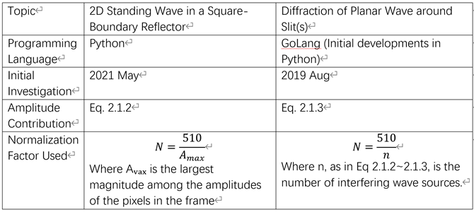
As mentioned in the Introduction, there are two projects that I have done using the point-sources simulation algorithm outlined in this article. They will constitute the coming parts of this series, some of their information are summarized in Img. 2.1.3